Data visualization for beginners – Part 2

Welcome to Part II of the series on data visualization. In the last blog post, we explored different ways to visualize continuous variables and infer information. If you haven’t visited that article, you can find it here. In this blog, we will expand our exploration to categorical variables and investigate ways in which we can visualize and gain insights from them, in isolation and in combination with variables (both categorical and continuous).

Before we dive into the different graphs and plots, let’s define a categorical variable. In statistics, a categorical variable is one which has two or more categories, but there is no intrinsic ordering to them, for example, gender, color, cities, age group, etc. If there is some kind of ordering between the categories, the variables are classified as ordinal variables, for example, if you categorize car prices by cheap, moderate and expensive. Although these are categories, there is a clear ordering between the categories.

# Importing the necessary libraries.  
import numpy as np  
import pandas as pd  
import seaborn as sns  
import matplotlib.pyplot as plt  
%matplotlib inline  

We will be using the Adult data set, which is an extraction of the 1994 census dataset. The prediction task is to determine whether a person makes more than 50K a year. Here is the link to the dataset. In this blog, we will be using the dataset only for data analysis.

# Since the dataset doesn't contain the column header, we need to specify it manually.   
cols = ['age', 'workclass', 'fnlwgt', 'education', 'education-num', 'marital-status', 'occupation', 'relationship', 'race', 'gender', 'capital-gain', 'capital-loss', 'hours-per-week', 'native-country', 'annual-income']  

# Importing dataset   
data = pd.read_csv('adult dataset/adult.data', names=cols)  

# The first five columns of the dataset.   
data.head()  

Bar graph

A bar chart or graph is a graph with rectangular bars or bins that are used to plot categorical values. Each bar in the graph represents a categorical variable and the height of the bar is proportional to the value represented by it.

Bar graphs are used:

• To make comparisons between variables
• To visualize any trend in the data, i.e., they show the dependence of one variable on another
• Estimate values of a variable

# Let's start by visualizing the distribution of gender in the dataset.  
fig, ax = plt.subplots()  
x = data.gender.unique()  
# Counting 'Males' and 'Females' in the dataset  
y = data.gender.value_counts()  
# Plotting the bar graph  
ax.bar(x, y)  
ax.set_xlabel('Gender')  
ax.set_ylabel('Count')  
plt.show()  

From the figure, we can infer that there are more number of males than females in the dataset. Next, we will use the bar graph to visualize the distribution of annual income based on both gender and hours per week (i.e. the number of hours they work per week). 

# For this plot, we will be using the seaborn library as it provides more flexibility with dataframes.   
sns.barplot(data.gender, data['hours-per-week'], hue=data['annual-income'])  
plt.show()

So from the figure above, we can infer that males and females with annual income less than 50K tend to work more per week.

Countplot

This is a seaborn-specific function which is used to plot the count or frequency distribution of each unique observation in the categorical variable. It is similar to a histogram over a categorical rather than quantitative variable.

So, let’s plot the number of males and females in the dataset using the countplot function.

# Using Countplot to count number of males and females in the dataset.  
sns.countplot(data.gender)  
plt.show()  

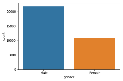
Earlier, we plotted the same thing using a bar graph, and it required some external calculations on our part to do so. But we can do the same thing using the countplot function in just a single line of code. Next, we will see how we can use countplot for deeper insights.

# ‘hue’ is used to visualize the effect of an additional variable to the current distribution.  
sns.countplot(data.gender, hue=data['annual-income'])  
plt.show()  

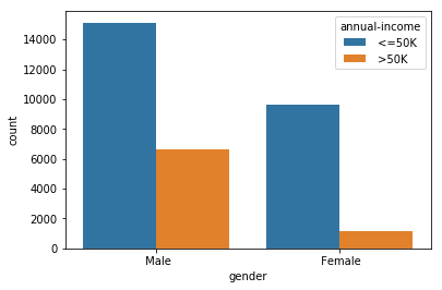
From the figure above, we can count that number of males and females whose annual income is <=50 and > 50K. We can see that the approximate number of

• Males with annual income <=50K : 15,000
• Males with annual income > 50K: 7000
• Females with annual income <=50K: 9000
• Females with annual income > 50K: 1000

So, we can infer that out of 32,500 (approx) people, only 8000 people have income greater than 50K, out of which only 1000 of them are females.

Box plot

Box plots are widely used in data visualization. Box plots, also known as box and whisker plots are used to visualize variations and compare different categories in a given set of data. It doesn’t display the distribution in detail but is useful in detecting whether a distribution is skewed and detect outliers in the data. In a box and whisker plot:

• the box spans the interquartile range
• a vertical line inside the box represents the median
• two lines outside the box, the whiskers, extending to the highest and the lowest observations represent the possible outliers in the data

Let’s use a box and whisker plot to find a correlation between ‘hours-per-week’ and ‘relationship’ based on their annual income.

# Creating a box plot  
fig, ax = plt.subplots(figsize=(15, 8))  
sns.boxplot(x='relationship', y='hours-per-week', hue='annual-income', data=data, ax=ax)  
ax.set_title('Annual Income of people based on relationship and hours-per-week')  
plt.show()  

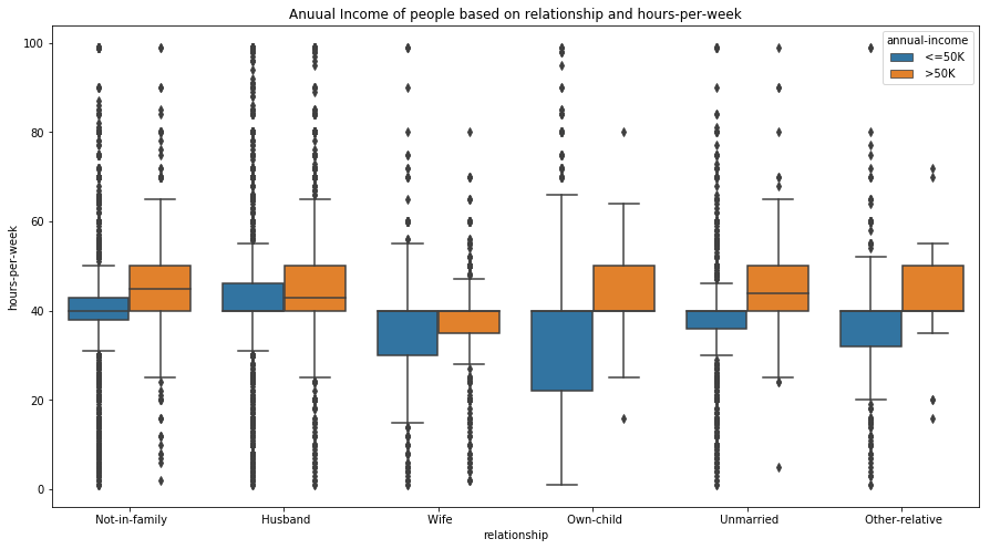
We can interpret some interesting results from the box plot. People with the same relationship status and an annual income more than 50K often work for more hours per week. Similarly, we can also infer that people who have a child and earn less than 50K tend to have more flexible working hours.
Apart from this, we can also detect outliers in the data. For example, people with relationship status ‘Not in family’ (see Fig 6.) and an income less than 50K have a large number of outliers at both the high and low ends. This also seems to be logically correct as a person who earns less than 50K annually may work more or less depending on the type of job and employment status.

Strip plot

Strip plot is a data analysis technique used to plot the sorted values of a variable along one axis. It is used to represent the distribution of a continuous variable with respect to the different levels of a categorical variable. For example, a strip plot can be used to show the distribution of the variable ‘gender’, i.e., males and females, with respect to the number of hours they work each week. A strip plot is also a good complement to a box plot or a violin plot in cases where you want to showcase all the observations along with some representation of the underlying distribution.

# Using Strip plot to visualize the data.  
fig, ax= plt.subplots(figsize=(10, 8))  
sns.stripplot(data['annual-income'], data['hours-per-week'], jitter=True, ax=ax)  
ax.set_title('Strip plot')  
plt.show()  

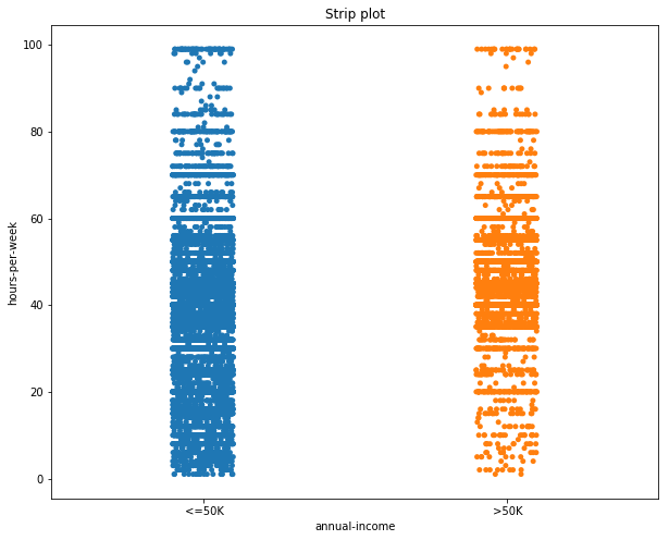
In the figure, by looking at the distribution of the data points, we can deduce that most of the people with an annual income greater than 50K work between 40 and 60 hours per week. While those with income less than 50K work can work between 0 and 60 hours per week.

Violin plot

Sometimes the mean and median may not be enough to understand the distribution of the variable in the dataset. The data may be clustered around the maximum or minimum with nothing in the middle. Box plots are a great way to summarize the statistical information related to the distribution of the data (through the interquartile range, mean, median), but they cannot be used to visualize the variations in the distributions.

A violin plot is a combination of a box plot and kernel density function (KDE, described in Part I of this blog series) which can be used to visualize the probability distribution of the data. Violin plots can be interpreted as follows:

• The outer layer shows the probability distribution of the data points and indicates 95% confidence interval. The thicker the layer, the higher the probability of the data points, and vice-versa.
• The second layer shows a box plot indicating the interquartile range.
• The third layer, or the dot, indicates the median of the data.

  

Let’s now build a violin plot. To start with, we will analyze the distribution of annual income of the people w.r.t. the number of hours they work per week.

fig, ax = plt.subplots(figsize=(10, 8))  
sns.violinplot(x='annual-income', y='hours-per-week', data=data, ax=ax)  
ax.set_title('Violin plot')  
plt.show()  

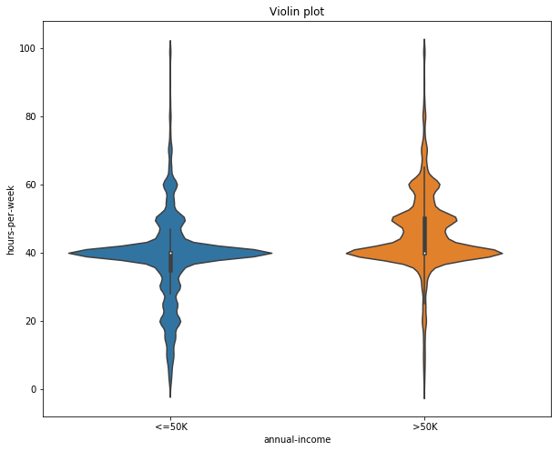
In Fig 9, the median number working hours per week is same (40 approximately) for both people earning less than 50K and greater than 50K. Although people earning less than 50K can have a varied range of the hours they spend working per week, most of the people who earn more than 50K work in the range of 40 – 80 hours per week.

Next, we can visualize the same distribution, but this grouping them according to their gender.

# Violin plot  
fig, ax = plt.subplots(figsize=(10, 8))  
sns.violinplot(x='annual-income', y='hours-per-week', hue='gender', data=data, ax=ax)  
ax.set_title('Violin plot grouped according to gender')  
plt.show()  

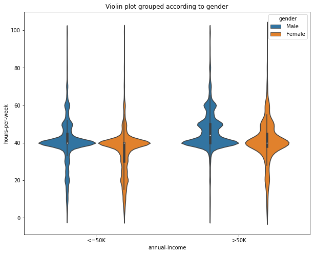
Adding the variable ‘gender’, gives us insights into how much each gender spends working per week based upon their annual income. From the figure, we can infer that males with annual income less than 50K tends to spend more hours working per week than females. But for people earning greater than 50K, both males and females spend an equal amount of hours per week working.

Violin plots, although more informative, are less frequently used in data visualization. It may be because they are hard to grasp and understand at first glance. But their ability to represent the variations in the data are making them popular among machine learning and data enthusiasts.

PairGrid

PairGrid is used to plot the pairwise relationship of all the variables in a dataset. This may seem to be similar to the pairplot we discussed in part I of this series. The difference is that instead of plotting all the plots automatically, as in the case of pairplot, Pair Grid creates a class instance, allowing us to map specific functions to the different sections of the grid.

Let’s start by defining the class.

# Creating an instance of the pair grid plot.  
g = sns.PairGrid(data=data, hue='annual-income')  

The variable ‘g’ here is a class instance. If we were to display ‘g’, then we will get a grid of empty plots. There are four grid sections to fill in a Pair Grid: upper triangle, lower triangle, the diagonal, and off-diagonal. To fill all the sections with the same plot, we can simply call ‘g.map’ with the type of plot and plot parameters.

# Creating a scatter plots for all pairs of variables.  
g = sns.PairGrid(data=data, hue='capital-gain')  
g.map(plt.scatter)  

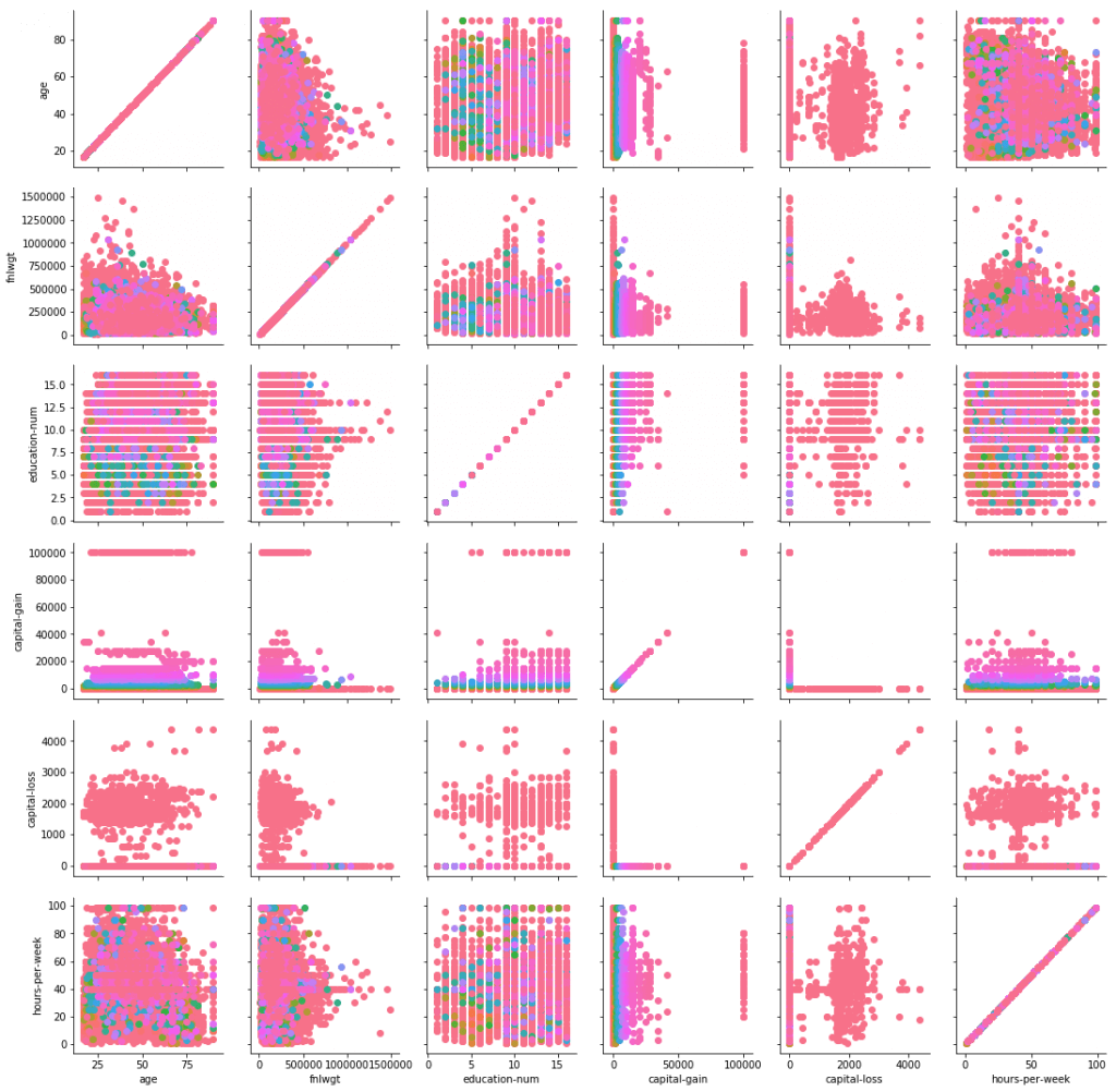
The ‘g.map_lower’ method only fills the lower triangle of the grid while the ‘g.map_upper’ method only fills the upper triangle of the grid. Similarly, ‘g.map_diag’ and ‘g.map_offdiag’ fills the diagonal and off-diagonal of the grid, respectively.

#Here we plot scatter plot, histogram and violin plot using Pair grid.  
g = sns.PairGrid(data=data, vars = ['age', 'education-num', 'hours-per-week'])  
# with the help of the vars parameter we can select the variables between which we want the plot to be constructed.  

g.map_lower(plt.scatter, color='red')  
g.map_diag(plt.hist, bins=15)  
g.map_upper(sns.violinplot)  

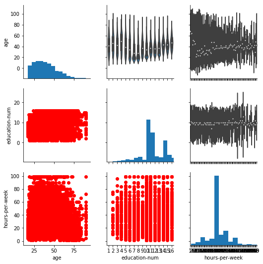
Thus with the help of Pair Grid, we can visualize the relationship between the three variables (‘hours-per-week’, ‘education-num’ and ‘age’) using three different plots all in the same figure. Pair grid comes in handy when visualizing multiple plots in the same figure.

Conclusion

Let’s summarize what we learned. So, we started with visualizing the distribution of categorical variables in isolation. Then, we moved on to visualize the relationship between a categorical and a continuous variable. Finally, we explored visualizing relationships when more than two variables are involved. Next week, we will explore how we can visualize unstructured data. Finally, I encourage you to download the given census data (used in this blog) or any other dataset of your choice and play with all the variations of the plots learned in this blog. Till then, Adiós!

Shubham Gupta Author 6 Blogs