Introduction
"The road to machine learning starts with Regression. Are you ready?"
If you are aspiring to become a data scientist, regression is the first algorithm you need to learn master. Not just to clear job interviews, but to solve real world problems. Till today, a lot of consultancy firms continue to use regression techniques at a larger scale to help their clients. No doubt, it's one of the easiest algorithms to learn, but it requires persistent effort to get to the master level.
Running a regression model is a no-brainer. A simple model <- y~x does the job. But optimizing this model for higher accuracy is a real challenge. Let's say your model gives adjusted R² = 0.678; how will you improve it?
In this article, I'll introduce you to crucial concepts of regression analysis with practice in R. Data is given for download below. Once you are finished reading this article, you'll able to build, improve, and optimize regression models on your own. Regression has several types; however, in this article I'll focus on linear and multiple regression.
Note: This article is best suited for people new to machine learning with requisite knowledge of statistics. You should have R installed in your laptops.
Table of Contents
- What is Regression? How does it work?
- What are the assumptions made in Regression?
- How do I know if these assumptions are violated in my data?
- How can I improve the accuracy of a Regression Model?
- How can I access the fit of a Regression Model?
- Practice Time - Solving a Regression Problem
What is Regression ? How does it work ?
Regression is a parametric technique used to predict continuous (dependent) variable given a set of independent variables. It is parametric in nature because it makes certain assumptions (discussed next) based on the data set. If the data set follows those assumptions, regression gives incredible results. Otherwise, it struggles to provide convincing accuracy. Don't worry. There are several tricks (we'll learn shortly) we can use to obtain convincing results.
Mathematically, regression uses a linear function to approximate (predict) the dependent variable given as:
Y = βo + β1X + ∈where,
Y - Dependent variable
X - Independent variable
βo - Intercept
β1 - Slope
∈ - Error
βo and β1 are known as coefficients. This is the equation of simple linear regression. It's called 'linear' because there is just one independent variable (X) involved. In multiple regression, we have many independent variables (Xs). If you recall, the equation above is nothing but a line equation (y = mx + c) we studied in schools. Let's understand what these parameters say:
Y - This is the variable we predict
X - This is the variable we use to make a prediction
βo - This is the intercept term. It is the prediction value you get when X = 0
β1 - This is the slope term. It explains the change in Y when X changes by 1 unit. ∈ - This represents the residual value, i.e. the difference between actual and predicted values.
Error is an inevitable part of the prediction-making process. No matter how powerful the algorithm we choose, there will always remain an (∈) irreducible error which reminds us that the "future is uncertain."
Yet, we humans have a unique ability to persevere, i.e. we know we can't completely eliminate the (∈) error term, but we can still try to reduce it to the lowest. Right? To do this, regression uses a technique known as Ordinary Least Square (OLS).
So the next time when you say, I am using linear /multiple regression, you are actually referring to the OLS technique. Conceptually, OLS technique tries to reduce the sum of squared errors ∑[Actual(y) - Predicted(y')]² by finding the best possible value of regression coefficients (β0, β1, etc).
Is OLS the only technique regression can use? No! There are other techniques such as Generalized Least Square, Percentage Least Square, Total Least Squares, Least absolute deviation, and many more. Then, why OLS? Let's see.
- It uses squared error which has nice mathematical properties, thereby making it easier to differentiate and compute gradient descent.
- OLS is easy to analyze and computationally faster, i.e. it can be quickly applied to data sets having 1000s of features.
- Interpretation of OLS is much easier than other regression techniques.
Let's understand OLS in detail using an example:
We are given a data set with 100 observations and 2 variables, namely Heightand Weight. We need to predict weight(y) given height(x1). The OLS equation can we written as:
Y = βo + β1(Height)+ ∈When using R, Python or any computing language, you don't need to know how these coefficients and errors are calculated. As a matter of fact, most people don't care. But you must know, and that's how you'll get close to becoming a master.
The formula to calculate these coefficients is easy. Let's say you are given the data, and you don't have access to any statistical tool for computation. Can you still make any prediction? Yes!
The most intuitive and closest approximation of Y is mean of Y, i.e. even in the worst case scenario our predictive model should at least give higher accuracy than mean prediction. The formula to calculate coefficients goes like this:
                        β1 = Σ(xi - xmean)(yi-ymean)/ Σ (xi - xmean)² where i= 1 to n (no. of obs.)

                       βo = ymean - β1(xmean)
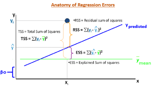
Now you know ymean plays a crucial role in determining regression coefficients and furthermore accuracy. In OLS, the error estimates can be divided into three parts:
Residual Sum of Squares (RSS) - ∑[Actual(y) - Predicted(y)]²
Explained Sum of Squares (ESS) - ∑[Predicted(y) - Mean(ymean)]²
Total Sum of Squares (TSS) - ∑[Actual(y) - Mean(ymean)]²
The most important use of these error terms is used in the calculation of the Coefficient of Determination (R²).
`R² = 1 - (SSE/TSS)`R² metric tells us the amount of variance explained by the independent variables in the model. In the upcoming section, we'll learn and see the importance of this coefficient and more metrics to compute the model's accuracy.
What are the assumptions made in regression ?
As we discussed above, regression is a parametric technique, so it makes assumptions. Let's look at the assumptions it makes:
- There exists a linear and additive relationship between dependent (DV) and independent variables (IV). By linear, it means that the change in DV by 1 unit change in IV is constant. By additive, it refers to the effect of X on Y is independent of other variables.
- There must be no correlation among independent variables. Presence of correlation in independent variables lead to Multicollinearity. If variables are correlated, it becomes extremely difficult for the model to determine the true effect of IVs on DV.
- The error terms must possess constant variance. Absence of constant variance leads to heteroskedestacity.
- The error terms must be uncorrelated i.e. error at
∈tmust not indicate the at error at∈t+1. Presence of correlation in error terms is known as Autocorrelation. It drastically affects the regression coefficients and standard error values since they are based on the assumption of uncorrelated error terms. - The dependent variable and the error terms must possess a normal distribution.
Presence of these assumptions make regression quite restrictive. By restrictive I meant, the performance of a regression model is conditioned on fulfillment of these assumptions.
How do I know these assumptions are violated in my data?
Once these assumptions get violated, regression makes biased, erratic predictions. I'm sure you are tempted to ask me, "How do I know these assumptions are getting violated?"
Of course, you can check performance metrics to estimate violation. But the real treasure is present in the diagnostic a.k.a residual plots. Let's look at the important ones:
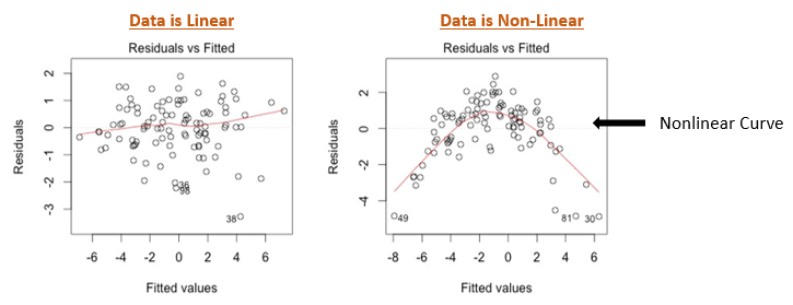
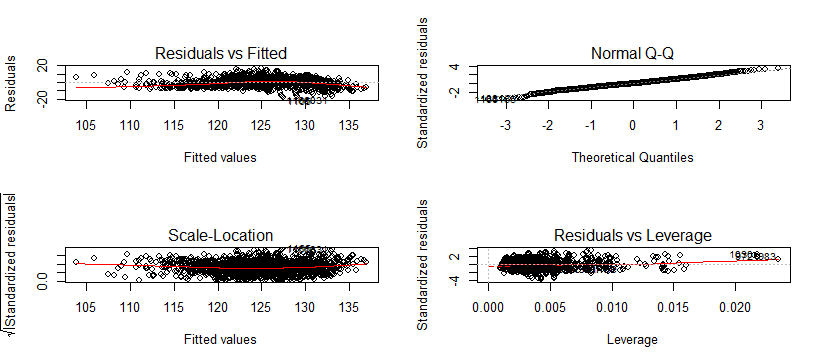
1. Residual vs. Fitted Values Plot
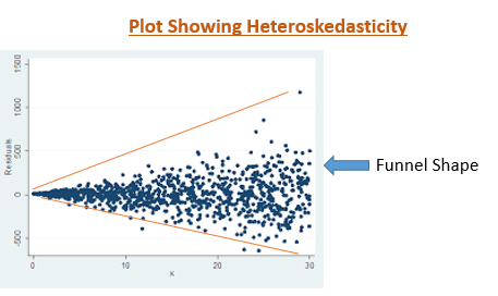
Ideally, this plot shouldn't show any pattern. But if you see any shape (curve, U shape), it suggests non-linearity in the data set. In addition, if you see a funnel shape pattern, it suggests your data is suffering from heteroskedasticity, i.e. the error terms have non-constant variance.
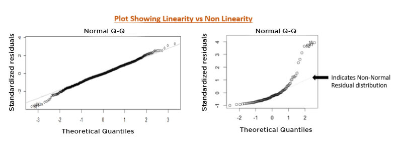
2. Normality Q-Q Plot
As the name suggests, this plot is used to determine the normal distribution of errors. It uses standardized values of residuals. Ideally, this plot should show a straight line. If you find a curved, distorted line, then your residuals have a non-normal distribution (problematic situation).
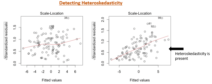
3. Scale Location Plot
This plot is also useful to determine heteroskedasticity. Ideally, this plot shouldn't show any pattern. Presence of a pattern determine heteroskedasticity. Don't forget to corroborate the findings of this plot with the funnel shape in residual vs. fitted values.
If you are a non-graphical person, you can also perform quick tests / methods to check assumption violations:
- Durbin Watson Statistic (DW) - This test is used to check autocorrelation. Its value lies between 0 and 4. A DW=2 value shows no autocorrelation. However, a value between 0 < DW < 2 implies positive autocorrelation, while 2 < DW < 4 implies negative autocorrelation.
- Variance Inflation Factor (VIF) - This metric is used to check multicollinearity. VIF <=4 implies no multicollinearity but VIF >=10 suggests high multicollinearity. Alternatively, you can also look at the tolerance (1/VIF) value to determine correlation in IVs. In addition, you can also create a correlation matrix to determine collinear variables.
- Breusch-Pagan / Cook Weisberg Test - This test is used to determine presence of heteroskedasticity. If you find p < 0.05, you reject the null hypothesis and infer that heteroskedasticity is present.
How can you improve the accuracy of a regression model ?
There is little you can do when your data violates regression assumptions. An obvious solution is to use tree-based algorithms which capture non-linearity quite well. But if you are adamant at using regression, following are some tips you can implement:
- If your data is suffering from non-linearity, transform the IVs using sqrt, log, square, etc.
- If your data is suffering from heteroskedasticity, transform the DV using sqrt, log, square, etc. Also, you can use weighted least square method to tackle this problem.
- If your data is suffering from multicollinearity, use a correlation matrix to check correlated variables. Let's say variables A and B are highly correlated. Now, instead of removing one of them, use this approach: Find the average correlation of A and B with the rest of the variables. Whichever variable has the higher average in comparison with other variables, remove it. Alternatively, you can use penalized regression methods such as lasso, ridge, elastic net, etc.
- You can do variable selection based on p values. If a variable shows p value > 0.05, we can remove that variable from model since at p> 0.05, we'll always fail to reject null hypothesis.
How can you access the fit of regression model?
The ability to determine model fit is a tricky process. The metrics used to determine model fit can have different values based on the type of data. Hence, we need to be extremely careful while interpreting regression analysis. Following are some metrics you can use to evaluate your regression model:
- R Square (Coefficient of Determination) - As explained above, this metric explains the percentage of variance explained by covariates in the model. It ranges between 0 and 1. Usually, higher values are desirable but it rests on the data quality and domain. For example, if the data is noisy, you'd be happy to accept a model at low R² values. But it's a good practice to consider adjusted R² than R² to determine model fit.
- Adjusted R²- The problem with R² is that it keeps on increasing as you increase the number of variables, regardless of the fact that the new variable is actually adding new information to the model. To overcome that, we use adjusted R² which doesn't increase (stays same or decrease) unless the newly added variable is truly useful.
- F Statistics - It evaluates the overall significance of the model. It is the ratio of explained variance by the model by unexplained variance. It compares the full model with an intercept only (no predictors) model. Its value can range between zero and any arbitrary large number. Naturally, higher the F statistics, better the model.
- RMSE / MSE / MAE - Error metric is the crucial evaluation number we must check. Since all these are errors, lower the number, better the model. Let's look at them one by one:
- MSE - This is mean squared error. It tends to amplify the impact of outliers on the model's accuracy. For example, suppose the actual y is 10 and predictive y is 30, the resultant MSE would be (30-10)² = 400.
- MAE - This is mean absolute error. It is robust against the effect of outliers. Using the previous example, the resultant MAE would be (30-10) = 20
- RMSE - This is root mean square error. It is interpreted as how far on an average, the residuals are from zero. It nullifies squared effect of MSE by square root and provides the result in original units as data. Here, the resultant RMSE would be √(30-10)² = 20. Don't get baffled when you see the same value of MAE and RMSE. Usually, we calculate these numbers after summing overall values (actual - predicted) from the data.
Solving a Regression Problem
Let's use our theoretical knowledge and create a model practically. As mentioned above, you should install R in your laptops. I've taken the data set from UCI Machine Learning repository. Originally, the data set is available in .txt file. To save you some time, I've converted it into .csv, and you can download it here.
Let's load the data set and do initial data analysis:
#set working directory
> path <- "C:/Users/Data/UCI"
> setwd(path)

#load data and check data
> mydata <- read.csv("airfoil_self_noise.csv")
> str(mydata)Sound_pressure_level as the dependent variable (to be predicted). In predictive modeling, we should always check missing values in data. If any data is missing, we can use methods like mean, median, and predictive modeling imputation to make up for missing data.
#check missing values
> colSums(is.na(mydata))> cor(mydata)Angle_of_Attack and Displacement show 75% correlation. It's up to us if we should consider this correlation % as a damaging level. Usually, correlation above 80% (subjective) is considered higher. Therefore, we can forego this combination and won't remove any variable.
In R, the base function lm is used for regression. We can run regression on this data by:
> regmodel <- lm(Sound_pressure_level ~ ., data = mydata)
> summary(regmodel)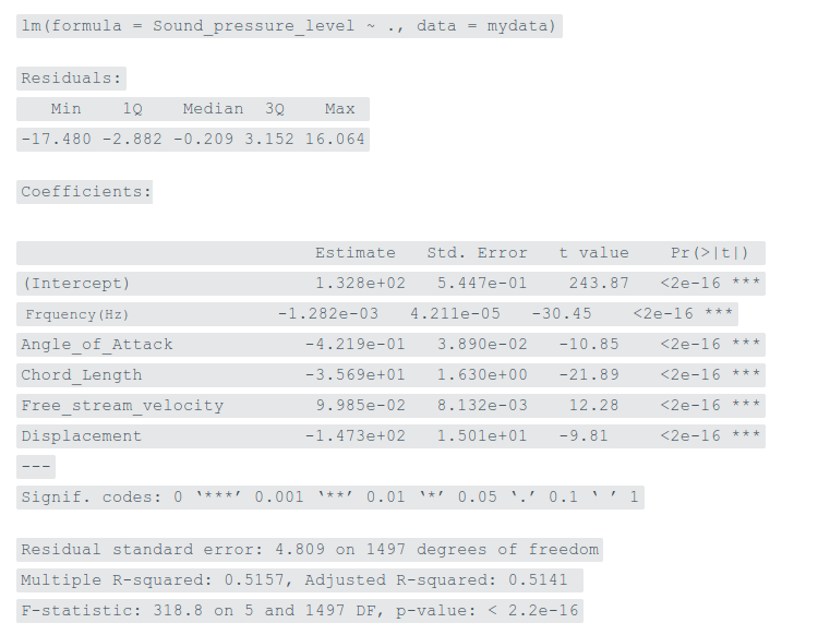
~ . tells lm to use all the independent variables. Let's understand the regression output in detail:
- Intercept - This is the βo value. It's the prediction made by model when all the independent variables are set to zero.
- Estimate - This represents regression coefficients for respective variables. It's the value of slope. Let's interpret it for
Chord_Length. We can say, whenChord_Lengthis increased by 1 unit, holding other variables constant,Sound_pressure_leveldecreases by a value of -35.69. - Std. Error - This determines the level of variability associated with the estimates. Smaller the standard error of an estimate is, more accurate will be the predictions.
- t value - t statistic is generally used to determine variable significance, i.e. if a variable is significantly adding information to the model. t value > 2 suggests the variable is significant. I used it as an optional value as the same information can be extracted from the p value.
- p value - It's the probability value of respective variables determining their significance in the model. p value < 0.05 is always desirable.
The adjusted R² implies that our model explains ~51% total variance in the data. And, the overall p value of the model is significant. Can we still improve this model ? Let's try to do it. Now, we'll check the residual plots, understand the pattern and derive actionable insights (if any):
> #set graphic output
> par(mfrow=c(2,2))

> #create residual plots
> plot (regmodel)
Among all, Residual vs. Fitted value catches my attention. Not exactly though, but I see signs of heteroskedasticity in this data. Remember funnel shape? You can see a similar pattern. To overcome this situation, we'll build another model with log(y).
> regmodel <- update(regmodel, log(Sound_pressure_level)~.)
> summary(regmodel)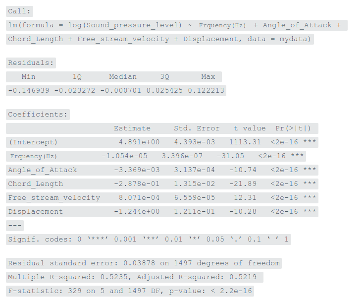
Though, the improvement isn't significant, we've increased our adjusted R² to 52.19%. Also, it looked like that funnel shape wasn't completely evident, thus implying non-severe effect of non-constant variance.
Let's divide the data set into train and test to check our final evaluation metric. We'll keep 70% data in train and 30% in test file. The reason being that we should keep enough data in train so that the model identifies obvious emerging patterns.
#sample
> set.seed(1)
> d <- sample ( x = nrow(mydata), size = nrow(mydata)*0.7)
> train <- mydata[d,] #1052 rows
> test <- mydata[-d,] #451 rows

#train model
> regmodel <- lm (log(Sound_pressure_level)~.,data = train)
> summary(regmodel)

#test model
> regpred <- predict(regmodel, test)

#convert back to original value
> regpred <- exp(regpred)

> library(Metrics)
> rmse(actual = test$Sound_pressure_level,predicted = regpred)
[1] 5.03423#save the output of boxplot
> d <- boxplot(train$Displacement,varwidth = T,outline = T,border = T,plot = T)
> d$out #enlist outlier observationsSummary
My motive in writing this article is to get you started at solving regression problems, with a greater focus on the theoretical aspects. Running an algorithm isn't rocket science, but knowing how it works will surely give you more control over what you do.
In this article, I've discussed the basics and semi-advanced concepts of regression. In addition, I've also explained best practices which you are advised to follow when facing low model accuracy. We learned about regression assumptions, violations, model fit, and residual plots with practical dealing in R. If you are a python user, you can run regression using linear.fit(x_train, y_train) after loading scikit learn library.
Did you find this tutorial helpful ? Let me know if there is anything you don't understand while reading this article. I'd love to answer your questions.

