Practical Guide to Clustering Algorithms & Evaluation in R

Introduction

Clustering algorithms are a part of unsupervised machine learning algorithms. Why unsupervised ? Because, the target variable is not present. The model is trained based on given input variables which attempt to discover intrinsic groups (or clusters).

As the target variable is not present, we can't label those groups. Then, how is it done? That's the interesting part we'll look at in this article!

Clustering algorithms are widely used across all industries such as retail, banking, manufacturing, healthcare, etc. In business terms, companies use them to separate customers sharing similar characteristics from others who don't to make customized engagement campaign strategies.

For example, in healthcare, a hospital might cluster patients based on their tumor size so that patients with different tumor sizes can be treated differently.

This technique helps us organize unstructured data. It can be used on tabular data, images, text data, etc. In this tutorial, we'll learn about clustering techniques, understand their working, and apply our newly gained knowledge on a data set.

Table of Contents

1. Types of Clustering Techniques
2. Distance Calculation for Clustering
3. K means Clustering | How does it work?
4. How to select the best value of k in k means?
5. Hierarchical Clustering | How does it work?
6. What are the evaluation methods used in cluster analysis?
7. Clustering in R - Water Treatment Plans

Types of Clustering Techniques

There are many types of clustering algorithms, such as K means, fuzzy c- means, hierarchical clustering, etc. Other than these, several other methods have emerged which are used only for specific data sets or types (categorical, binary, numeric).

Among these different clustering algorithms, there exists clustering behaviors known as

1. Soft Clustering: In this technique, the probability or likelihood of an observation being partitioned into a cluster is calculated.
2. Hard Clustering: In hard clustering, an observation is partitioned into exactly one cluster (no probability is calculated).

In this tutorial, we'll focus on the following techniques:

1. K means clustering
2. Hierarchical Clustering

Let's understand these techniques in detail. But before that, it's extremely crucial for you to get familiar with the distance metrics. These clustering techniques use distance measures to decide the similarity or dissimilarity in the observations.

It follows a simple rule: the closer the observations, the more similar they are, and vice versa.

Distance Calculation for Clustering

There are some important things you should keep in mind:

1. With quantitative variables, distance calculations are highly influenced by variable units and magnitude. For example, clustering variable height (in feet) with salary (in rupees) having different units and distribution (skewed) will invariably return biased results. Hence, always make sure to standardize (mean = 0, sd = 1) the variables. Standardization results in unit-less variables.
2. Use of a particular distance measure depends on the variable types; i.e., formula for calculating distance between numerical variables is different than categorical variables.

Suppose, we are given a 2-dimensional data with xi = (xi1, xi2, . . . , xip) and xj = (xj1, xj2, . . . , xjp). Both are numeric variables. We can calculate various distances as follows:

1. Euclidean Distance: It is used to calculate the distance between quantitative (numeric) variables. As it involves square terms, it is also known as L2 distance (because it squares the difference in coordinates). Its formula is given by

                    d(xi , xj ) = (|xi1 − xj1|² + |xi2 − xj2|² + . . . + |xip − xjp|² ) 1/2

2. Manhattan Distance: It is calculated as the absolute value of the sum of differences in the given coordinates. This is known as L1 distance. It is also sometimes called the Minowski Distance.

An interesting fact about this distance is that it only calculates the horizontal and vertical distances. It doesn't calculate the diagonal distance. For example, in chess, we use the Manhattan distance to calculate the distance covered by rooks. Its formula is given by:

                    d(xi , xj ) = (|xi1 − xj1| + |xi2 − xj2| + . . . + |xip − xjp|

3. Hamming Distance: It is used to calculate the distance between categorical variables. It uses a contingency table to count the number of mismatches among the observations. If a categorical variable is binary (say, male or female), it encodes the variable as male = 0, female = 1.

In case a categorical variable has more than two levels, the Hamming distance is calculated based on dummy encoding. Its formula is given by (x,y are given points):

                      hdist(x, y) <- sum((x[1] != y[1]) + (x[2] != y[2]) + ...)

Here, a != b is defined to have a value of 1 if the expression is true, and a value of 0 if the expression is false. This is also known as the Jaccard Coefficient.

4. Gower Distance: It is used to calculate the distance between mixed (numeric, categorical) variables. It works this way: it computes the distance between observations weighted by its variable type, and then takes the mean across all variables.

Technically, the above-mentioned distance measures are a form of Gower distances; i.e. if all the variables are numeric in nature, Gower distance takes the form of Euclidean. If all the values are categorical, it takes the form of Manhattan or Jaccard distance. In R, ClusterOfVar package handles mixed data very well.

5. Cosine Similarity: It is the most commonly used similarity metric in text analysis. The closeness of text data is measured by the smallest angle between two vectors. The angle (Θ) is assumed to be between 0 and 90. A quick refresher: cos (Θ = 0) = 1 and cos (Θ = 90) = 0.

Therefore, the maximum dissimilarity between two vectors is measured at Cos 90 (perpendicular). And, two vectors are said to be most similar at Cos 0 (parallel). For two vectors (x,y), the cosine similarity is given by their normalized dot product shown below:

                     cossim(x, y) <- dot(x, y)/(sqrt(dot(x,x)*dot(y,y)))

Let's understand the clustering techniques now.

K means Clustering | How does it work ?

This technique partitions the data set into unique homogeneous clusters whose observations are similar to each other but different than other clusters. The resultant clusters remain mutually exclusive, i.e., non-overlapping clusters.

In this technique, "K" refers to the number of cluster among which we wish to partition the data. Every cluster has a centroid. The name "k means" is derived from the fact that cluster centroids are computed as the mean distance of observations assigned to each cluster.

This k value k is given by the user. It's a hard clustering technique, i.e., one observation gets classified into exactly one cluster.

Technically, the k means technique tries to classify the observations into K clusters such that the total within cluster variation is as small as possible. Let C denote a cluster. k denotes the number of clusters. So, we try to minimize:

                      minimum(Cι..Cκ){∑W(Cκ)}

But, how do we calculate within cluster variation? The most commonly used method is squared Euclidean distance. In simple words, it is the sum of squared Euclidean distance between observations in a cluster divided by the number of observations in a cluster (shown below): 

|Cκ| denotes the number of observations in a cluster.

Now, we fairly understand what goes behind k means clustering. But how does it start ? Practically, it takes the following steps:

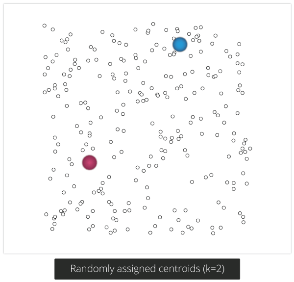
1. Let's say the value of k = 2. At first, the clustering technique will assign two centroids randomly in the set of observations.
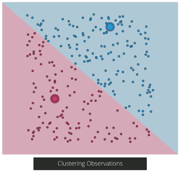
2. Then, it will start partitioning the observations based on their distance from the centroids. Observations relatively closer to any centroid will get partitioned accordingly.
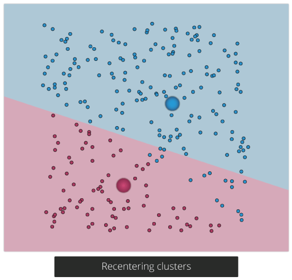
3. Then, based on the number of iterations (after how many times we want the algorithm to converge) we've given, the cluster centroids will get recentered in every iteration. With this, the algorithm will try to continually optimize for the lowest within cluster variation.
4. Based on the newly assigned centroids, assign each observation falling closest to the new centroids.
5. This process continues until the cluster centers do not change or the stopping criterion is reached.

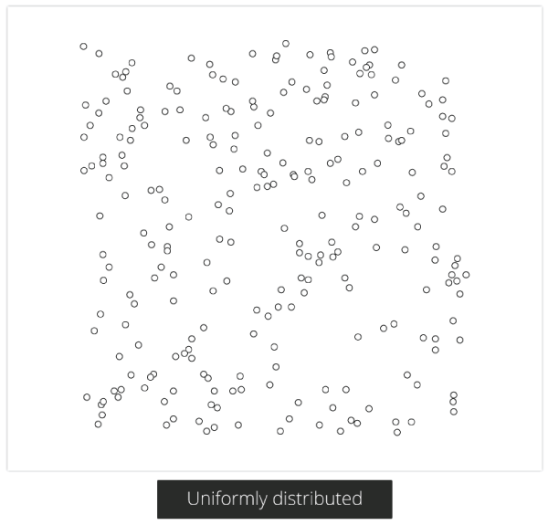
The visual explanation of the these steps can be seen below:

Hopefully, now you'd have a better understanding of k means clustering.

How to select best value of k in k means?

Determining the best value of k plays a critical role in k means model performance. To select best value of k, there is no "one rule applies all situation." It depends on the shape and distribution of the observations in a data set.

Intuitively, by finding the best value of k, we try to find a balance between the number of clusters and the average variation within a cluster.

Following are the methods useful to find an optimal k value:

1. Cross Validation: It's a commonly used method for determining k value. It divides the data into X parts. Then, it trains the model on X-1 parts and validates (test) the model on the remaining part.

The model is validated by checking the value of the sum of squared distance to the centroid. This final value is calculated by averaging over X clusters. Practically, for different values of k, we perform cross validation and then choose the value which returns the lowest error.

2. Elbow Method: This method calculates the best k value by considering the percentage of variance explained by each cluster. It results in a plot similar to PCA's scree plot. In fact, the logic behind selecting the best cluster value is the same as PCA.

In PCA, we select the number of components such that they explain the maximum variance in the data. Similarly, in the plot generated by the elbow method, we select the value of k such that percentage of variance explained is maximum.

3. Silhouette Method: It returns a value between -1 and 1 based on the similarity of an observation with its own cluster. Similarly, the observation is also compared with other clusters to derive at the similarity score. High value indicates high match, and vice versa. We can use any distance metric (explained above) to calculate the silhouette score.

4. X means Clustering: This method is a modification of the k means technique. In simple words, it starts from k = 1 and continues to divide the set of observations into clusters until the best split is found or the stopping criterion is reached. But, how does it find the best split ? It uses the Bayesian information criterion to decide the best split.

Hierarchical Clustering | How does it work ?

In simple words, hierarchical clustering tries to create a sequence of nested clusters to explore deeper insights from the data. For example, this technique is being popularly used to explore the standard plant taxonomy which would classify plants by family, genus, species, and so on.

Hierarchical clustering technique is of two types:

1. Agglomerative Clustering – It starts with treating every observation as a cluster. Then, it merges the most similar observations into a new cluster. This process continues until all the observations are merged into one cluster. It uses a bottoms-up approach (think of an inverted tree).

2. Divisive Clustering – In this technique, initially all the observations are partitioned into one cluster (irrespective of their similarities). Then, the cluster splits into two sub-clusters carrying similar observations. These sub-clusters are intrinsically homogeneous. Then, we continue to split the clusters until the leaf cluster contains exactly one observation. It uses a top-down approach.

Here we’ll study about agglomerative clustering (it's the most commonly used).

This technique creates a hierarchy (in a recursive fashion) to partition the data set into clusters. This partitioning is done in a bottoms-up fashion. This hierarchy of clusters is graphically presented using a Dendogram (shown below).

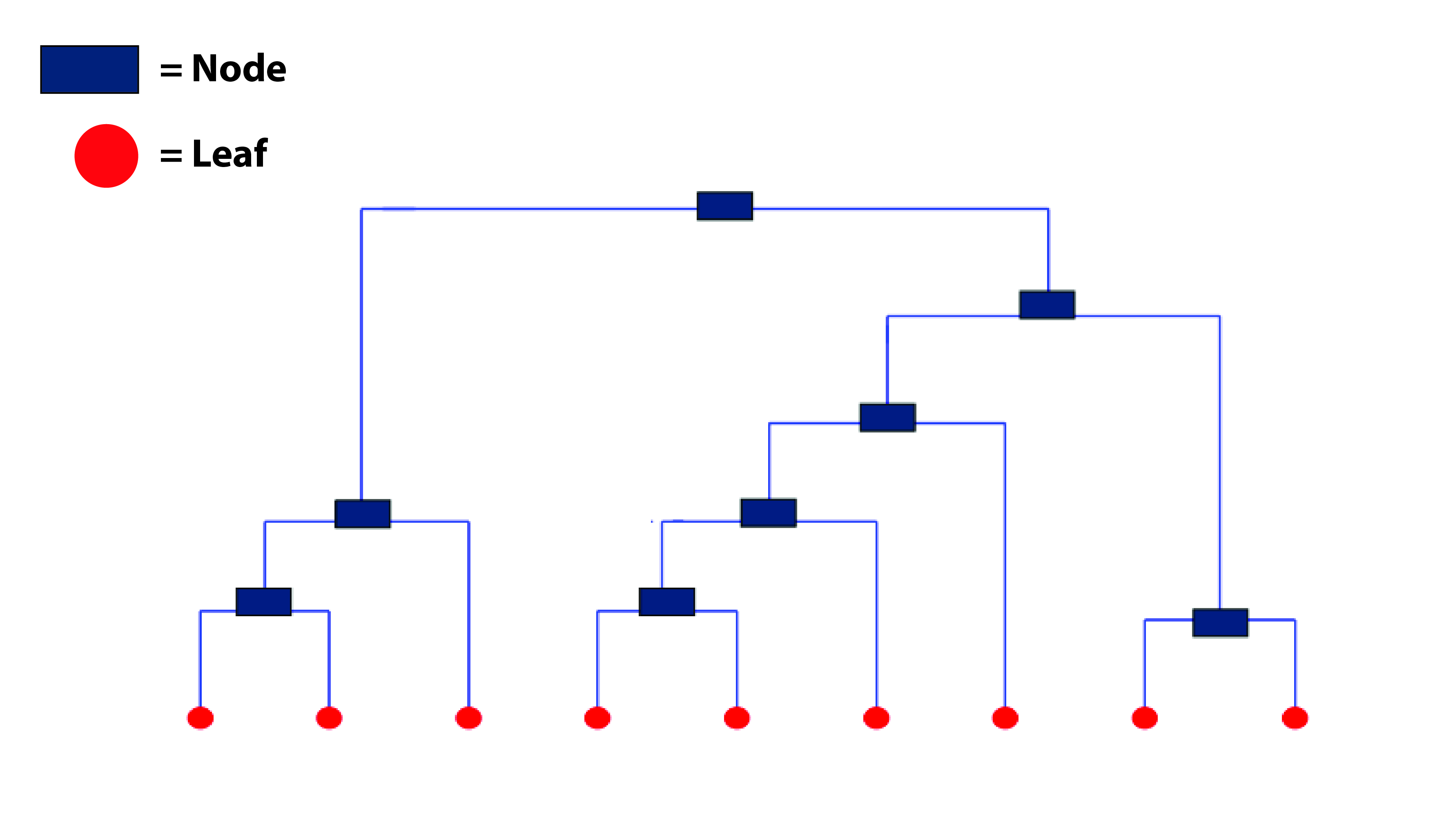
This dendrogram shows how clusters are merged / split hierarchically. Each node in the tree is a cluster. And, each leaf of the tree is a singleton cluster (cluster with one observation). So, how do we find out the optimal number of clusters from a dendrogram?

Let’s understand how to study a dendrogram.

As you know, every leaf in the dendrogram carries one observation. As we move up the leaves, the leaf observations begin to merge into nodes (carrying observations which are similar to each other). As we move further up, these nodes again merge further.

Always remember, lower the merging happens (towards the bottom of the tree), more similar the observations will be. Higher the merging happens (toward the top of the tree), less similar the observations will be.

To determine clusters, we make horizontal cuts across the branches of the dendrogram. The number of clusters is then calculated by the number of vertical lines on the dendrogram, which lies under horizontal line.

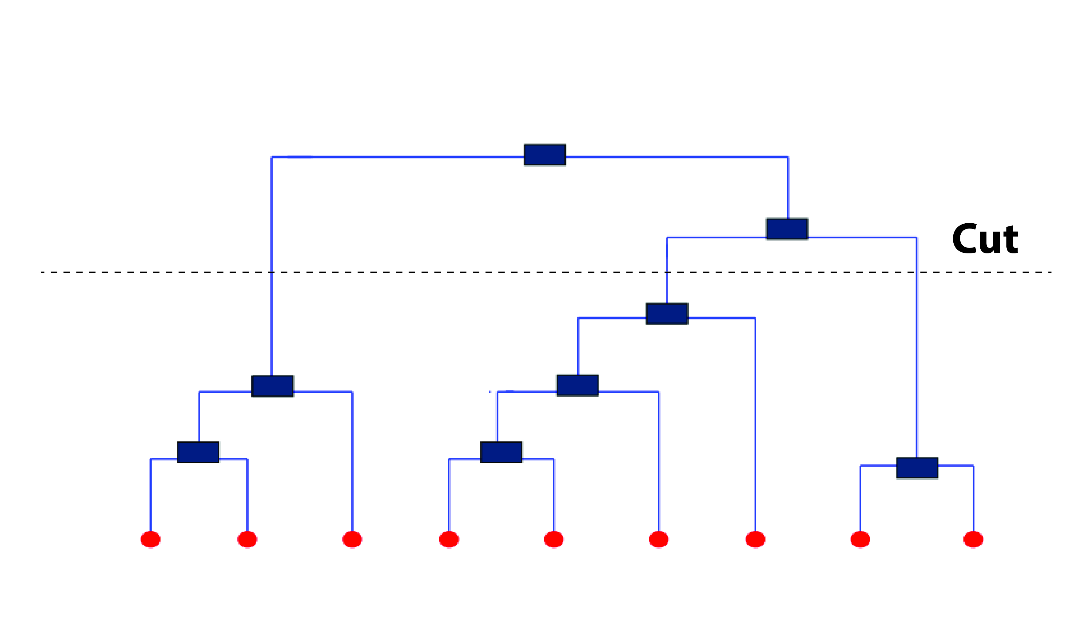
As seen above, the horizontal line cuts the dendrogram into three clusters since it surpasses three vertical lines. In a way, the selection of height to make a horizontal cut is similar to finding k in k means since it also controls the number of clusters.

But, how to decide where to cut a dendrogram? Practically, analysts do it based on their judgement and business need. More logically, there are several methods (described below) using which you can calculate the accuracy of your model based on different cuts. Finally, select the cut with a better accuracy.

The advantage of using hierarchical clustering over k means is, it doesn't require advanced knowledge of number of clusters. However, some of the advantages which k means has over hierarchical clustering are as follows:

• It uses less memory.
• It converges faster.
• Unlike hierarchical, k means doesn't get trapped in mistakes made on a previous level. It improves iteratively.
• k means is non-deterministic in nature, i.e.. after every time you initialize, it will produce different clusters. On the contrary, hierarchical clustering is deterministic.

Note: K means is preferred when the data is numeric. Hierarchical clustering is preferred when the data is categorical.

What are the evaluation methods used in cluster analysis ?

In supervised learning, we are given a target variable to calculate the model's accuracy. But, what do you do when there is no target variable? How can we benchmark the model's performance? The methods to evaluate clustering accuracy can be divided into two broad categories:

*Internal Accuracy Measures: *As the name suggests, these measures calculate the cluster's accuracy based on the compactness of a cluster. Following are the methods which fall under this category:

1. Sum of Squared Errors (SSE) - The compactness of a cluster can be determined by calculating its SSE. It works best when the clusters are well separated from one another. Its formula is given by (shown below) where Cκ is the number of observations in a cluster. µκ is the mean distance in cluster k.

2. Scatter Criteria - In simple words, it calculates the spread of a cluster. To do that, first it calculates a scatter matrix, within cluster scatter and between cluster scatter. Then, it sums over the resulting values to derive total scatter values. Lower values are desirable. Let's understand their respective formulas:

The scatter matrix is the  sum of [product of (difference between the observation and its cluster mean) and (its transpose)]. It is calculated by

Within cluster scatter (Sω) is simply the sum of all Sκ values. The between cluster matrix (SB) can be calculated as

where Nκ is the number of observations in the k cluster and µ is the total mean vector calculated as

where m is the number of matches in the cluster. Finally, the total scatter metric S(T) can be calculated as

                        S(T) = Sω + SΒ

*External Accuracy Measures: *These measures are calculated by matching the structure of the clusters with some pre-defined classification of instances in the data. Let's look at these measures:

1. Rand Index - It compares the two clusters and tries to find the ratio of matching and unmatched observations among two clustering structures (C1 and C2). Its value lies between 0 and 1. Think of the clustering structures (C1 and C2) with several small clusters. Think of C1 as your predicted cluster output and C2 as the actual cluster output. Higher the value, better the score. Its simple formula is given by:

RAND SCORE = a + d / (a + b + c + d)

where

• a = observations which are available in the same cluster in both structures (C1 and C2)
• b = observations which are available in a cluster in C1 and not in the same cluster in C2
• c = observations which are available in a cluster in C2 and not in the same cluster in C1
• d = observations which are available in different clusters in C1 and C2

2. Precision Recall Measure -  This metric is derived from the confusion matrix. Recall is also known as Sensitivity [True Positive/ (True Positive + False Negative)]. For clustering, we use this measure from an information retrieval point of view. Here, precision is a measure of correctly retrieved items. Recall is measure of matching items from all the correctly retrieved items.

Clustering in R - Water Treatment Plants

Let's now work on a data set and understand clustering in a practical way. Understanding the concept is important, coding is the easy part. I've taken the data set from UCI Machine Learning repository. For your convenience, the data is also available for download here.

This data set consists of sensor activity measurement from an urban waster water treatment plant. Our task is to cluster the data based on an operational order such that the organization can understand more about its chances of failure. All the variables are numeric in nature.

Let's start with hierarchical clustering. You can get more information on data here. Before reaching the clustering stage, let's quickly get over with the basic data pre-processing steps.

#set working directory
> path <- "data/Cluster_Tutorial" > setwd(path)

#load libraries
> library(data.table)
> library(ggplot2)
> library(fpc)

#load data
> water_data <- read.table("water-treatment.data.txt",sep = ",",header = F,na.strings = c("?"))
> setDT(water_data)
> head(water_data)

As you see, the variable 'V1' is a categorical variable which will help us identifying which cluster contains which value. Since, rest are numeric values we'll have to scale them prior to doing clustering.

#lets check missing values
> colSums(is.na(water_data))

Some of the variables have missing values. Let's impute the missing values with median.

#impute missing values with median
> for(i in colnames(water_data)[!(colnames(water_data) %in% c("V1"))])
set(x = water_data,i = which(is.na(water_data[[i]])), j = i, value = median(water_data[[i]], na.rm = T))

#scale the variables
> scaled_wd <- scale( water_data[,-c("V1"),with=F])

Now, our data is ready for clustering! For hierarchical clustering, we'll first calculate a distance matrix based on Euclidean measure. Then using the hclust function, we can implement hierarchical clustering.

#Hierarchical Clustering
> d <- dist(scaled_wd, method = "euclidean")

#distance matrix
> h_clust <- hclust(d, method = "ward") #clustering

#dendrogram
> plot(h_clust,labels = water_data$V1)

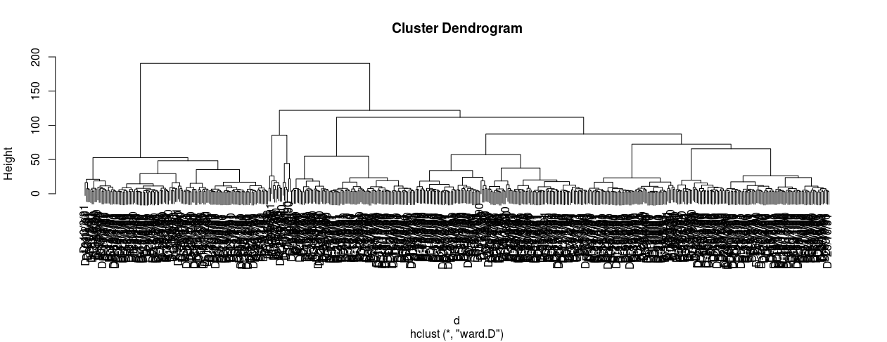
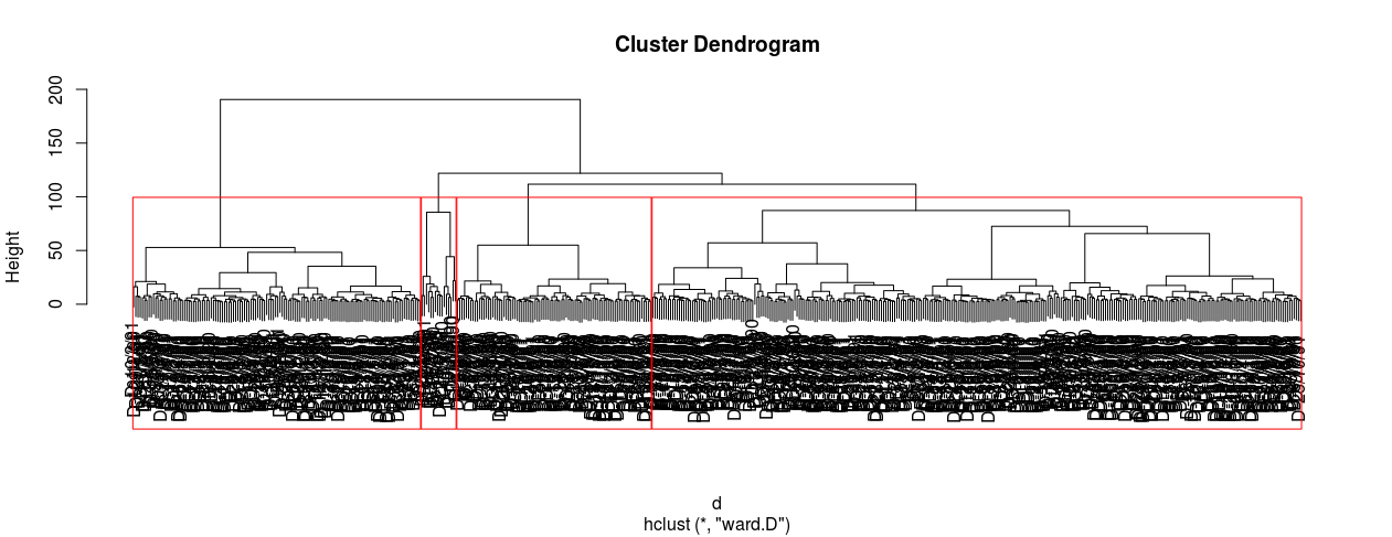
I hope you can understand this dendrogram now. All the leaves at the bottom carry one observation each, which are then merged into similar values as they rise upward. Now, how can you estimate the number of clusters? Going by the logic of horizontal cut, four clusters are evident. Let's see!

> rect.hclust(h_clust,k=4)

To look at which observation went into which cluster, you can write:

#extract clusters
> groups <- cutree(h_clust,k=4)
> groups

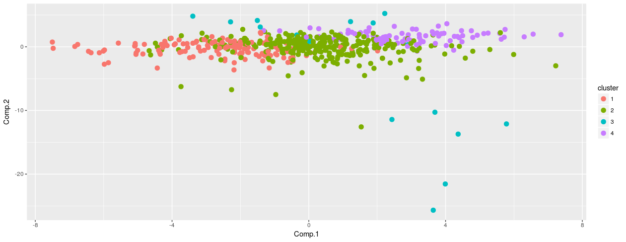
Let's visualize the clusters in a better way. However, visualizing this high dimensional data in one plot has its own challenges. A smart way could be, to visualize the cluster on principal components of this data. This way we would be able to capture most of information by reducing the data dimension.

To implement PCA, we'll use princomp base function. For our convenience, we'll take only the first two components.

#pca
> pcmp <- princomp(scaled_wd)
> pred_pc <- predict(pcmp, newdata=scaled_wd)[,1:2]

Now, we'll create a data frame having pc values and their corresponding clusters. Then, using ggplot2 we'll create the plot.

> comp_dt <- cbind(as.data.table(pred_pc),cluster = as.factor(groups), Labels = water_data$V1)
> ggplot(comp_dt,aes(Comp.1,Comp.2))+ geom_point(aes(color = cluster),size=3)

Let's now proceed to k means clustering. We'll use the base function k means with 100 iterations to converge.

#kmeans
> kclust <- kmeans(scaled_wd,centers = 4,iter.max = 100)

You can check out the number of observations comprised by each cluster using kclust$size. Again, let's create a plot to understand this clustering better. The parameter kclust$cluster carries the information for the cluster label.

> ggplot(comp_dt,aes(Comp.1,Comp.2))+ geom_point(aes(color = as.factor(kclust$cluster)),size=3)

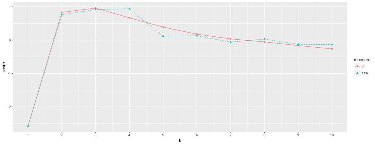
As seen above, both the techniques have partitioned the observations in same clusters. Is 4 the optimal number of clusters in k means ? Let's find out. To pick the best value of k, we'll use kmeansruns function from fpc package. This function is enabled with two distance metrics: Average silhouette width and Calinski-Harabasz. Let's try to use both the methods and check out the best k value.

> tunek <- kmeansruns(scaled_wd,krange = 1:10,criterion = "ch") > tunek$bestk #3
> tunekw <- kmeansruns(scaled_wd,krange = 1:10,criterion = "asw") > tunekw$bestk #4

Finally, let's plot the k value against distance score.

Summary

In supervised learning problems, clustering offers a fantastic opportunity for feature engineering. Isn't it?

Apart from k means, hierarchical clustering, there are other clustering techniques such as association mining. Association mining helps a lot in bundling products in a shopping store. Hence, it's being widely used in the retail industry. It's an interesting topic which we shall cover in future articles.

In this tutorial, we learned about clustering techniques from scratch. We started with covering the fundamentals of clustering followed by getting hands-on experience in performing cluster analysis in R.

Did you like this tutorial? Feel free to drop in your comments, suggestions, and share your experience while dealing with clustering problems.